AP 186 Activity 4 - Length and Area Estimation in Images

 
In this activity, we will use Green's theorem and its discrete form is what I am gonna use is[1]:

where N_b is the number of pixels in the boundary of our shape, x_i and y_i are the pixel locations of the boundary of our shape.


I made three images in Paint where the background is black and the shape is white. I saved the images as a monochrome bitmap (*.bmp) so that I will not convert the image into grayscale. The images are a triangle, a circle, and a rectangle.

Figure 1. Image of a triangle used in the activity.

Figure 2. Image of a circle used in the activity.

Figure 3. Image of a rectangle used in the activity.

Using Scilab 5.4.1 with SIVP and IPD toolboxes, I read the image and then used the function edge(E1, 'canny'). To use edge, you must first have the SIVP - Scilab Image and Video Processing Toolbox. To find the pixel locations of the edges, I used the find function. To show what edge does to the images, I used ShowImage() to see the results.

Figure 4. Resulting image of edge function to triangle image.

Figure 5. Resulting image of edge function to circle image.

Figure 6. Resulting image of edge function to rectangle image.

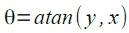
Now I have to find the center of the shapes, and I did that by getting the sum of the edge pixel locations of x and then dividing it by the number of edge pixel locations of x. The same was done in the edge pixel location of y to get the edge pixel location of the center of the edge shape for the y-coordinate.  The x center pixel coordinate of the edge shape was then subtracted from the pixel coordinates of x, and the same was done to the y pixel coordinates of the edge shape. This was done so that we can get the angle theta by using the equation:

 

and then using equation:

to sort the [x,y] pixel locations in an increasing order. To do this, I used the gsort function in Scilab. Now that it has been sorted in increasing angle, I will now use Green's theorem. I used a for loop to get the difference inside the bracket then placed it in a matrix with the same size as the number of pixels minus one. I then used the sum function to the matrix, then multiplied it to 0.5 to get the area of the shape in the image.

I need to compare this to the analytic value of the area of these shapes to check if what I did was right. At first, I didn't know how to do this so I looked at the data of the original image. I saw that it was mostly in zeros but luckily I saw a column with some values of 255. What would that mean? This must be because the image is expressed as a pixel value. The white pixels should be 255, and the black pixels will be 0 so I have to find only the white pixels. So when I found the white pixels in the original image using the find function, then the column size of that resulting matrix will be the area of the shape since they are the total of all the white pixels in the original image. The summary of my results are on the table below.

.
The lowest percent error was in the rectangle, then the circle. The highest percent error goes to the triangle. These percent error are very low and I must say that my results are very accurate. My code which used Scilab is shown below. It used the discrete form of Green's theorem to calculate the area.

Figure 7. Part 1 of my Scilab code to get area using Green's theorem.

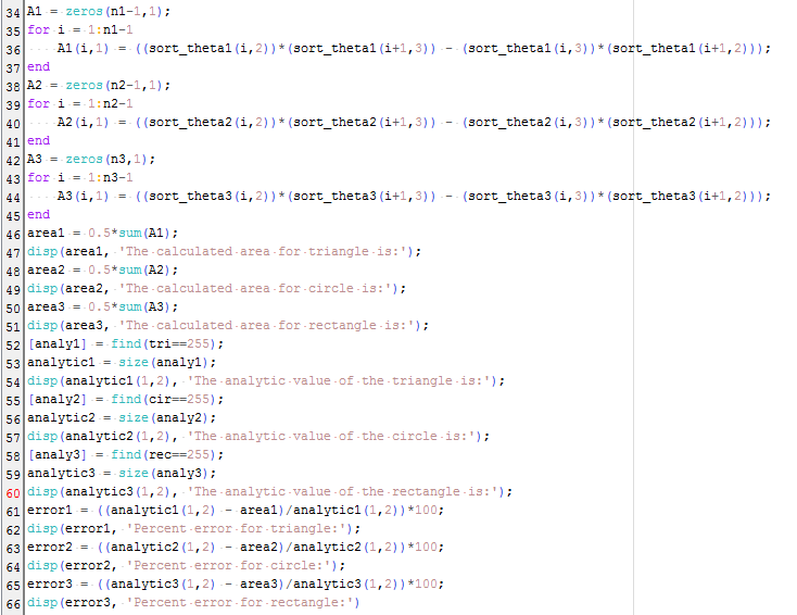Figure 8. Part 2 of my Scilab code to get area using Green's theorem.

Figure 9. Map of Trinoma mall taken from Google Maps. At the lower rightmost edge is the scale.

I will now apply our technique to an irregular shape and to do that I used a specific place in Google Maps which is Trinoma mall. I used the setting of terrain in Google Maps so that I can clearly see the boundaries of the location. We know that there is a scale in Google Maps which is 100 meters, I measured this 100 meters in the image and I got 85 pixels. This means that for every 85 pixels in the image, there are 100 meters in the physical coordinates.

 I delineated the boundaries of Trinoma by making the background black and the lot shape of Trinoma to be white like I used in the images in the first part. I saved this as monochrome bitmap so that I will not convert it from color to grayscale. I did the same process as I did with the shapes before and the edge image of Trinoma is shown below.

Figure 10. Delineated monochrome bitmap image of Trinoma map.

Figure 11. Resulting image of Trinoma map using edge function.

The calculated area of this edge image of Trinoma is 203,398 pixels squared. Converting this to meter squared, we get 146450 meters squared. To check the accuracy of my measurement, I searched for Trinoma's lot size and I got 20 hectares or 200,000 meters squared [2]. A percent error of 27 % was calculated by using the actual value of Trinoma's lot size. The percent error of Trinoma was noticeably high compared to the other shapes. As I recall, the triangle shape has the largest percent error of the three shapes and that must be one of the resaons why it is large. I also think that because the shape is irregular, Green's theorem will have a higher error compared to the shapes that I did.
Here is my Scilab code:

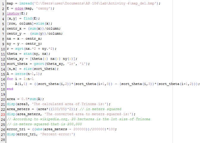Figure 12. Scilab code for area estimation of Trinoma.

ImageJ is a java-based, free image processing software that was developed by the National Institutes of Health,US to measure microscopic images. We use this software to measure any length on an image by setting the scale of known value into it. We do this by scanning an object, in this case, a LRT-2 stored value card and measuring one of its dimensions. I chose to measure its width using a ruler and I got 5.4 cm. I opened the LRT-2 card image into ImageJ and used the straight-line tool to make a horizontal line from one end of the image to another. To set the scale, from the menu bar click Analyze then Set Scale. I entered the known distance, 5.4 cm, then put the unit which is in centimeters or cm. The pixel ratio must be 1.0 and the distance in pixels is the value of the line in pixels that you had drawn. This will set the scale and you can measure any line or polygon using ImageJ by clicking Measure in the menu bar and choosing Analyze. This will give parameters like area, mean, min, max, angle and length of any part of the image. When I created a line to the length of the card, and used Measure then Analyze, I got a value of 8.445 cm. I measured the value of the length using a ruler and I got 8.55 cm. I got a percent error of 1.228% when I compared these two values.

For the area, the actual area that I got which is the product of my measured values is 46.17 cm squared. Using ImageJ's polygon tool and Analyze, I got a value of 44.984 cm squared. The percent error that I got is  2.569 %. I think that this percent error versus the measured values are small so ImageJ is an accurate and  helpful tool to measure some things when you know one dimension of it. But this is only applicable for two dimensions, so a flat object like this LRT-2 card is ideal.

Figure 12. Scanned picture of a LRT-2 card. 

If I will grade myself in this activity, I will give myself a 10 since I did the code and I discovered how to get the analytic value of the area which for a long time was my biggest question throughout this activity. I also enjoyed using ImageJ and solving for the area either analytic or using Green's theorem.


References:
  [1]  M. Soriano, AP 186 Activity Manual, Activity 4 Length and area estimation in images, 2014.
  [2] Wikipedia.org, http://en.wikipedia.org/wiki/TriNoma