AP 186 Activity 6 - Properties and Applications of the 2D Fourier Transform

So we now apply the basics of Fourier transform and see how it is used in image processing.

Part A. Anamorphic Property of FT of different 2D patterns.

We are asked to get the Fourier transform(FT) of the following:

a) Tall rectangular aperture

b) Wide rectangular aperture

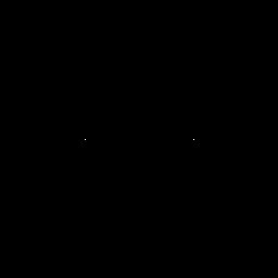
c) Two dots along x-axis

d) Same as c) but different spacing

I did all the images (a,b,c,d) in GIMP. What I did is is got the FT of the image and then displayed its modulus. I used fftshift to make sure the output image is in the right quadrant.

Figure 1. Tall rectangular aperture.

Figure 2. FT of tall rectangular aperture.

 The FT of the tall rectangular aperture has a bright wide rectangle in the center and some interference pattern on its sides. 

Figure 3. Wide rectangular aperture.

Figure 4. FT of wide rectangular aperture.

The wide rectangular aperture's FT is opposite of the FT of the tall rectangular aperture.

Now, two dots along x-axis with equal spacing. We take its FT and we get the image in Figure 6.

Figure 5. Two dots along x-axis.

Figure 6. FT of the two dots.

The FT of the two dots looks like a sinusoid along the x-direction.
 Now, same as the two dots but different spacing:

Figure 7. Two dots on the center but different spacing. 

And the FT of the figure above: 

Figure 8. FT of figure 9. 

As we can see the sinusoid along x-direction has increased in frequency.

This time, the same dots with wider spacing than Figure 9.

Figure 11. Two dots with widest spacing.

Figure 12. FT of figure 11.

This shows that as the spacing between the dots increases, the frequency of the FT transform increases.

Part B. Rotation property of FT.

So first I created a 2D sinusoid in the x-direction in Scilab using this code:

nx = 128; ny = 128;

x = linspace(-1,1,nx);

y = linspace(-1,1,ny);

[X,Y] = ndgrid(x,y);

f = 4 //frequency – you may change this later.

z = sin(2*%pi*f*X)

(Y*sin(theta2) + X*cos(theta2)));

h = scf();

grayplot(x,y,z');

h.color_map = hotcolormap(32);

And then I cropped the picture of the plot and it will be converted into grayscale when I run my code for Fourier transform(FT). 

Figure 13. 2D sinusoid in the x-direction with frequency = 4.

Figure 14. FT of 2D sinusoid with frequency = 4.

Now, what happens when we increase the frequency?

Figure 15. Image of 2D sinusoid with frequency = 6(left) and FT of the sinusoid(right).

Figure 16. Image of 2D sinusoid with frequency = 8(left) and FT of the sinusoid(right).

Figure 17. Image of 2D sinusoid with frequency = 10(left) and FT of the sinusoid(right).

Figure 18. FT of the 2D sinusoids (a) with frequency =4, (b) frequency = 6, (c) frequency =8, (d) frequency = 10.

As we can see as the frequency increases the spacing between the center dot and the two other dots are increasing.  This looks like the effect of the two dots with different spacing but the opposite, in the two dots with spacing, the FT is the sinusoid, while here the FT is the image of three dots and we can see that the frequency and spacing of the two other dots in reference to the center dot are directly proportional.

 Figure 18. 2D sinusoid with constant bias (left) and FT of the sinusoid (right). 

So suppose you have an image of an interferogram from Young's double slit experiment? So what I did was knowing the frequencies of the sinusoids in Figures 15-17, I measured the distance in pixels from the top of the white pixel to the top of the gray pixel above, and from the bottom of the white pixel to the end of the bottom gray pixel in Figure 18. I notice that this pixel distance, when you divide it by 2, you get the frequency of the sinusoid.  I did the same thing to the one with constant bias, and I got the value of the constant bias. So this is what you can do to measure the frequency of the interferogram, you can get the distance between the two slits(until the end of the slits), then divide it by two, you can get the frequency.

We now rotate our sinusoid and this happens.

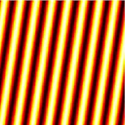
Figure 19. Rotated sinusoid with angle = 30degrees (left) and its FT (right).

Figure 20. Combination of sinusoids in X and Y (left) and its FT(right).

For the rotated sinusoid with an angle of 30 degrees, you can see that the rotation in the FT is opposite of direction with respect to the source image. So the combination of sinusoids in X and Y have a center dot and dots like the ends of a square around it.

So then, we are asked to add rotated sinusoids into Figure 20's sinusoid image. We have to predict the FT of this image. So my prediction it is rotated (counterclockwise) with 4 gray points around a brightest point in center. Let us see if I am right.

Figure 21. Combination of sinusoids in X and Y with rotated sinusoids (left) and its FT(right).

So my prediction was right but there are more than four gray points around the brightest point.

Filtering in Fourier space

Part C. Convolution Theorem Redux

We take the Fourier transform(FT) modulus of the two dots with a size of one pixel each which is symmetric to the center. These two dots are like Dirac deltas.

Figure 22. Two dots with and its FT modulus (right).

Now we replace the two dots with two circles.

Figure 23. Two circles (left) and its FT modulus (right).

Figure 24. Two circles with wider radius (left) and its FT modulus (right).

Figure 25. Two circles with the widest radius of the three (left) and its FT modulus (right).

 So the pattern is like sinusoids along x-axis mixed with the Airy disks. We can see that as the radius increases, the Airy disk's(center disk) radius decreases. This is like the previous blog post, where as the radius of the circular aperture increases, the diffraction pattern (or FT pattern) decreases which is a property of FT. I think this happens because the FT modulus of two Dirac deltas along x-axis symmetric to the center is sinusoids along x-axis and the FT of a circular aperture is the Airy disk. This output is a convolution of two Dirac deltas and the circular aperture. 

Now we change the two dots with two squares.

Figure 26. Two squares symmetric to center (left) and its FT modulus (right).

And we increase the width of our squares.

Figure 30. Two squares with bigger width (left) and its FT modulus (right).

Figure 31. Two squares with biggest width of the three (left) and its FT modulus (right).

Like the previous example of the two circles, now we see the combination of sinusoids along x-axis with the FT modulus of a square aperture. As the width of the squares increases, the diffraction pattern of the square aperture decreases that is a property of FT. This pattern is the convolution of the two Dirac deltas and square aperture.

Now we make two Gaussians using the equation

 and this time with mu_naught as the peak position and sigma squared is the variance.

Figure 32. Two Gaussians with variance of 0.0001 (left) and its FT modulus (right).

Figure 33. Two Gaussians with variance of 0.0025 (left) and its FT modulus (right).

Figure 34. Two Gaussians with variance of 0.0081 and its FT modulus(right).

As we can see the FT of a Gaussian is like a circular aperture which has an Airy disk pattern and the FT of the two Dirac deltas is sinusoids along the x-axis. This is a combination of the two so we can say that this pattern is a convolution of the two Dirac deltas and a Gaussian.

Now, I will create a 200x200 array full of zeros. I will add ten 1's to this array randomly, I will call this matrix A. This is the result. And I assigned an arbitrary 3x3 matrix which I assigned to be d = [1 0 0;0 1 0; 0 0 1] in Scilab. I convolved matrix A and d, and the result is in the figure below.

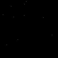
Figure 35. The matrix A(left) and the convolution of A and d (right).

Now we take the FT modulus of equally spaced 1's in 200x200 matrix of zeros. We will increase the spacing between the dots which I will call width. 

Figure 36. Grid used with width = 5 and its FT (right).

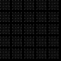
Figure 37. Grid used with width = 10 and its FT(right).

Figure 38. Grid used with width = 50 and its FT (right).

Figure 39. Grid used with width = 100 and its FT (right).

As the width or spacing between the input grid increases, so does the dots in the FT of the grid. So the one's are like the Dirac deltas, the if they are many in an equally spaced matrix and you take its FT, it will look like figure 35 (right).

 For Part D. Fingerprint filtering.
I took a picture of my fingerprint and I converted it into grayscale using Scilab. I proceeded to taking its FT and to see the frequencies of the fingerprint edges lie I used the log scale. Its FT is shown below.

 Figure 40. My fingerprint and its FT shown using log scale.

And I made the mask in GIMP, and I prioritized the center bright spot and my mask is like an annulus which is shown in figure 39. I customized the mask using GIMP since it is not a perfect circle and I want to capture the peak frequencies of the fingerprint.

Figure 41. Mask made from FT(Left) and (right) FT of fingerprint in log scale.

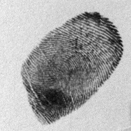
Figure 42. Grayscale image of my fingerprint (left) and filtered image (right). 

As you can see the ridges of the fingerprint are more pronounced and the blotches are lessened. I used the mask and fftshifted it, then multiplied it to the fftshifted FT of the grayscale image. I used inverse FFT to get the image back and rotated it so the orientation will be like the original image.

For part E. Lunar landing image.

The same steps were used as the fingerprint but the peak frequencies to be blocked are much more easier. 

Figure 43. Original lunar landing image taken from [1].

Figure 44. Grayscale of the original image (left) and its FT in log scale. 

So we know that the peak frequencies of the grayscale image are in the horizontal and vertical x-axis. We have to preserve the center of the FT in log scale. So the mask is like this:

Figure 45. Mask (right) and FT in log scale of image (right).

This mask is that so we can filter the vertical lines as well as the other horizontal lines in the picture.

Figure 46. Grayscale of the original image of lunar (left) and filtered image (right).

Now it looks very good compared to the grayscale of the original image. I was really amazed when I saw it! I spent a large amount of time to do this since I was confused on how to use the mask at first. In my attempts, I got the same image. So how did I do it? I fftshifted the mask and multiplied it to the fftshifted FT of the grayscale image. I used the inverse FT then rotated the output image since the inverse FT flips the image. I really liked the output image since the vertical lines take out the focus on how beautiful the moon surface is. 

Part F. Canvas weave pattern.

Now, the we try to filter out the canvas weave pattern in our photo. 

Figure 46. Detail of an oil painting from the UP Vargas museum collection.

Figure 47. Grayscale of the original image. 

So we take again the FT of the grayscale image in log scale and we got:

Figure 48. FT of image in logscale.

Figure 49. Mask made in GIMP.

So the peak frequencies are the dots around the center of the FT in log scale and I designed the mask so that it will block it. So now the output image was made by multiplying the fftshifted mask and fftshifted FT of the grayscale image, applying inverse FT and rotating the image so the orientation is the same as the original image. So we now compare the grayscale and the filtered output image.

Figure 50. Grayscale of original image.

Figure 51. Filtered image. 

As you can see the canvas weave pattern is gone! Now we can appreciate the painting more because the focus is on the painting not on its canvas weave pattern.

Now we invert the colors of our mask:

Figure 52. Inverted colors of mask used for removal of canvas weave.

And then we take its inverse FT and the result is:

Figure 53. Inverse FT of inverted mask.

Wow! It is an Airy disk! But what is the pattern inside the Airy disk? It resembles the canvas weave pattern that we removed from the painting! You can now see the pattern that you filtered out in the canvas weave pattern.

I will give myself a score of 10/10 for trying hard and getting the required images right. I really worked hard and sometimes the debugging the code frustrates me but it was worth it. I learned a lot and the outputs were amazing. I can't believe the changes will be dramatic but they are. Filtering using FT is a very useful tool and I feel like I'm so cool cause I did it!

Thank you very much to Ma'am Jing Soriano for helping me out understand about the constant and non-constant bias and cheering me on my debate in MBB 1! Thank you very much to Kat Bulan, Ritz Aguilar and Pam Pasion. Our discussions made me head on the right direction with filtering the images.

References:
[1] M. Soriano, Applied Physics 186 manual, A6 - Properties and Applications of the 2D Fourier Transform, 2014.